Linear Circuit Analysis
1. Introduction
2. Basic Concepts
- Charge, current, and voltage
- Power and energy
- Linear circuits
- Linear components
- Nodes and loops
- Series and parallel
- R, L & C combinations
- V & I combinations
3. Simple Circuits
- Ohm's law
- Kirchhoff's current law
- Kirchhoff's voltage law
- Single loop circuits
- Single node-pair circuits
- Voltage division
- Current division
4. Nodal and Mesh Analysis (DC)
5. Additional Analysis Techniques (DC)
- Superposition
- Source transformation
- The $V_{test}/I_{test}$ method
- Norton equivalent
- Thévenin equivalent
- Max power transfer
- DC analysis of L & C
6. AC Analysis
7. Magnetically Coupled Circuits
8. Polyphase Systems
9. Operational Amplifiers
10. Laplace Transforms
11. Time-Dependent Circuits
- Introduction
- Inductors and capacitors
- First-order transients
- Second-order transients
-
Parallel RLC circuits
Series RLC circuits - Nodal analysis
- Mesh analysis
- Laplace transforms
- Additional techniques
12. Two-Port Networks
Appendix
Python
Python is a powerful, high-level programming language known for its simplicity, versatility, and readability. It usually comes preinstalled on most Linux systems, however, it is not installed by default on most macOS or Windows systems. On these systems it is recommended to install Python manually from python.org.
Due to its extensive standard library and vast ecosystem of third-party packages Python is a versatile tool in linear circuit analysis, in particular for solving circuit equations in the DC, AC, or time domain, analyzing frequency response, and visualizing results. This section provides a brief introduction to using Python for solving both linear and nonlinear equations. In CircuitsU, users can often export the system of equations (particularly in nodal or mesh analysis) to a Python script file and run it locally on their computer for further exploration and analysis.
Solving Systems of Algebraic Equations
There are multiple ways to solve systems of algebraic equations in Python. If the system is linear, you can use the NumPy library to
input the matrix and the right-hand side vector, and then use the numpy.linalg.solve() function to find the solution.
If the system is nonlinear, you can use the SciPy library's fsolve() function, which is designed to find the roots of a system of nonlinear equations.
However, the method that is often the easiest to use in linear circuit analysis is the SymPy library, which allows for symbolic mathematics
and can handle both linear and nonlinear equations. Another advantage of SymPy is that you do not need to convert the equations to matrix form; you can
input them directly, as shown in the examples below.
Example 1
Compute the sought variables for the circuit below using nodal analysis.
import sympy as sp

# Define variables
v1, v2, v3, v4, V0, Pg = sp.symbols('v1 v2 v3 v4 V0 Pg')

# Define equations
eq1 = sp.Eq((v1-v3)/2+(v1-v2)/9-9, 0)
eq2 = sp.Eq((v2-v1)/9+2+(v2-v4)/3, 0)
eq3 = sp.Eq(v3/20+(v3-v1)/2, 0)
eq4 = sp.Eq(-(2)+v4/3+(v4-v2)/3, 0)
eq5 = sp.Eq(V0, v4-v2)
eq6 = sp.Eq(Pg, -9*(0-v1))

# Solve system of equations
solutions = sp.solve((eq1, eq2, eq3, eq4, eq5, eq6), (v1, v2, v3, v4, V0, Pg))

print(solutions)
Example 2
Compute the sought variables for the circuit below using mesh analysis.
import sympy as sp

# Define variables
i1, i2, i3, Vx, I0 = sp.symbols('i1 i2 i3 Vx I0')

# Define equations
eq1 = sp.Eq(5*Vx, i1-i3)
eq2 = sp.Eq(10*(i2-i1)+3*i2, 0)
eq3 = sp.Eq(-4+2*i3+10*i3+10*(i1-i2), 0)
eq4 = sp.Eq(Vx, -2*i3)
eq5 = sp.Eq(I0, i2)

# Solve system of equations
solutions = sp.solve((eq1, eq2, eq3, eq4, eq5), (i1, i2, i3, Vx, I0))

print(solutions)
Example 3
In the case of AC circuits, use sp.I for the imaginary complex number $j$, like in the example below.
import sympy as sp

# Define variables
i1, i2, I0 = sp.symbols('i1 i2 I0')

# Define equations
eq1 = sp.Eq(sp.I*13*i1+4*(i1-i2)+(1+5*sp.I), 0)
eq2 = sp.Eq(-(3+4*sp.I)+(-sp.I*1)*i2+4*(i2-i1), 0)
eq3 = sp.Eq(I0, i1)

# Solve system of equations
solutions = sp.solve((eq1, eq2, eq3), (i1, i2, I0))

print(solutions)
Plotting in Python
Matplotlib is the most popular and foundational plotting library in Python. It is great for 2D plots such line plots, scatter plots, histograms, bar charts, contour plots, etc.
Simple Plots
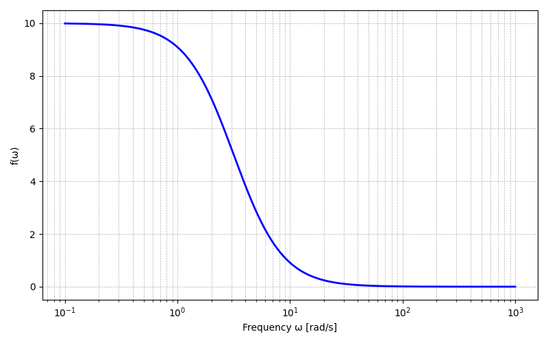
For instance, let's plot $$\begin{equation} f(\omega)=100/(\omega^2+10) \end{equation}$$ using a log scale on the x-axis.
import numpy as np
import matplotlib.pyplot as plt

# 1. Define frequency range (logarithmic scale)
w = np.logspace(-1, 3, 1000)   # ω from 0.1 to 1000 (rad/s)

# 2. Define function f(ω) = 100 / (ω² + 10)
f = 100 / (w**2 + 10)

# 3. Plot on log scale (x-axis)
plt.figure(figsize=(8, 5))
plt.semilogx(w, f, color='blue', linewidth=2)
plt.xlabel('Frequency ω [rad/s]')
plt.ylabel('f(ω)')
plt.grid(which='both', linestyle='--', linewidth=0.5)
plt.tight_layout()
plt.show()
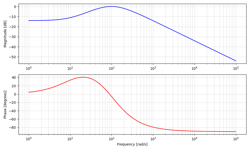
Magnitude and Angle Bode Plots (Real Poles and Zeros)
When making Bode plots it is convenient to use the signal library from scipy. For instance the code below draws the magnitude
and angle Bode plots of
$$\begin{equation} H(\class{mjblue}{j}\omega)=\frac{200(\class{mjblue}{j} \omega+10)}{(\class{mjblue}{j} \omega+100)^2} \end{equation}$$
import numpy as np
import matplotlib.pyplot as plt
from scipy import signal

# 1. Define transfer function: H(s) = 200 * (s + 10) / (s + 100)^2
num = [200, 2000]             # numerator = 200*s + 200
den = np.polymul([1, 100], [1, 100])  # denominator = (s + 100)^2
# den = [1, 200, 10000]

# 2. Compute frequency response
w = np.logspace(0, 5, 1000)   # frequency range: 10^0 → 10^5 rad/s
w, h = signal.freqs(num, den, w)

# 3. Plot magnitude and phase (Bode plot)
plt.figure(figsize=(10, 6))

# --- Magnitude (in dB) ---
plt.subplot(2, 1, 1)
plt.semilogx(w, 20 * np.log10(abs(h)), color='b')
plt.ylabel('Magnitude [dB]')
plt.grid(which='both', linestyle='--', linewidth=0.5)

# --- Phase (in degrees) ---
plt.subplot(2, 1, 2)
plt.semilogx(w, np.angle(h, deg=True), color='r')
plt.xlabel('Frequency [rad/s]')
plt.ylabel('Phase [degrees]')
plt.grid(which='both', linestyle='--', linewidth=0.5)

plt.tight_layout()
plt.show()
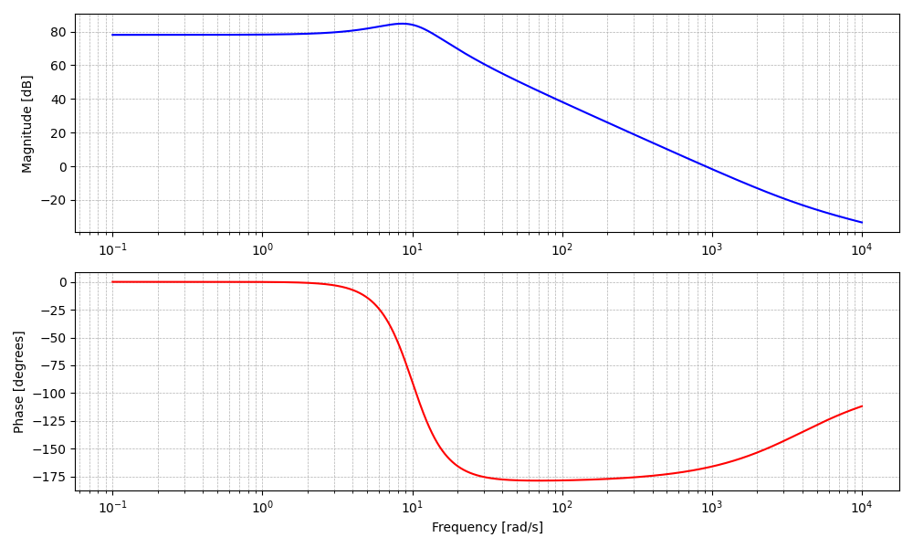
Magnitude and Angle Bode Plots (Complex Poles or Zeros)
When making Bode plots it is convenient to use the signal library from scipy. For instance the code below draws the magnitude
and angle Bode plots of
$$\begin{equation} H(\class{mjblue}{j}\omega)=\frac{200(\class{mjblue}{j} \omega+10)^2 (\class{mjblue}{j}\omega + 4000)}{(\class{mjblue}{j} \omega)^2+10(\class{mjblue}{j} \omega)+100} \end{equation}$$
        import numpy as np
import matplotlib.pyplot as plt
from scipy import signal

# 1. Define the transfer function: H(s) = 200 * (s + 10)^2 (s + 4000) / ((s^2 + 10s + 100)^2)

num = np.polymul(np.polymul(np.polymul([200],[1, 10]),[1, 10]),[1, 4000])  # Numerator: 200 * (s + 10)^2 * (s + 4000)
den = np.polymul([1, 10, 100] , [1, 10, 100] )  # Denominator: (s^2 + 10s + 100)^2

# 2. Frequency range and frequency response
w = np.logspace(-1, 4, 5000)  # ω from 0.1 to 1000 rad/s (log scale)
w, h = signal.freqs(num, den, w)

# 3. Plot magnitude and phase
plt.figure(figsize=(10, 6))

# --- Magnitude (dB) ---
plt.subplot(2, 1, 1)
plt.semilogx(w, 20 * np.log10(np.abs(h)), 'b')
plt.ylabel('Magnitude [dB]')
plt.grid(which='both', linestyle='--', linewidth=0.5)

# --- Phase (degrees) ---
plt.subplot(2, 1, 2)
plt.semilogx(w, np.angle(h, deg=True), 'r')
plt.xlabel('Frequency [rad/s]')
plt.ylabel('Phase [degrees]')
plt.grid(which='both', linestyle='--', linewidth=0.5)

plt.tight_layout()
plt.show()